
In my prior post, wherein I argued at length that US health care expenditures are reasonably well explained by Actual Individual Consumption (AIC) and that GDP is an inferior predictor, I pointed out toward the end that the linear specification I used is likely to significantly overstate US residuals because there is good evidence for non-linearity and because the US is far out on the frontier vis-a-vis consumption.
This non-linearity can be seen pretty clearly if you look at the 2011 data derived from the World Bank (for AIC) and WHO (for HCE).


Since some people may (1) doubt the accuracy of these statistics outside of the few highly developed countries (2) imagine that these poor countries are somehow qualitatively different in a way that’s not well correlated with their level of economic development or (3) are particularly reluctant to accept non-linearity as a potential partial explanation for the US here, I thought I’d approach this from a somewhat different angle.
I will analyze the OECD data for non-linearity using the entire time series. This gives me the opportunity to work around some of the limitations of having so few countries in any given year and in a relatively compressed range of at that. Further, I will exclude the United States from training data because it is presumably the only country that doesn’t have health care reasonably well figured out and I will exclude Luxembourg because it has a very large non-resident workforce (which skews per capita estimates in both dimensions). I will fit this with a 3rd degree polynomial since that appears to fit the broader 2011 WHO/WorldBank data better without the overfitting potential of loess (especially amongst the tails).

(Note: blue=loess, green=poly3,black=poly2)
First off, let’s just plot the OECD time series data: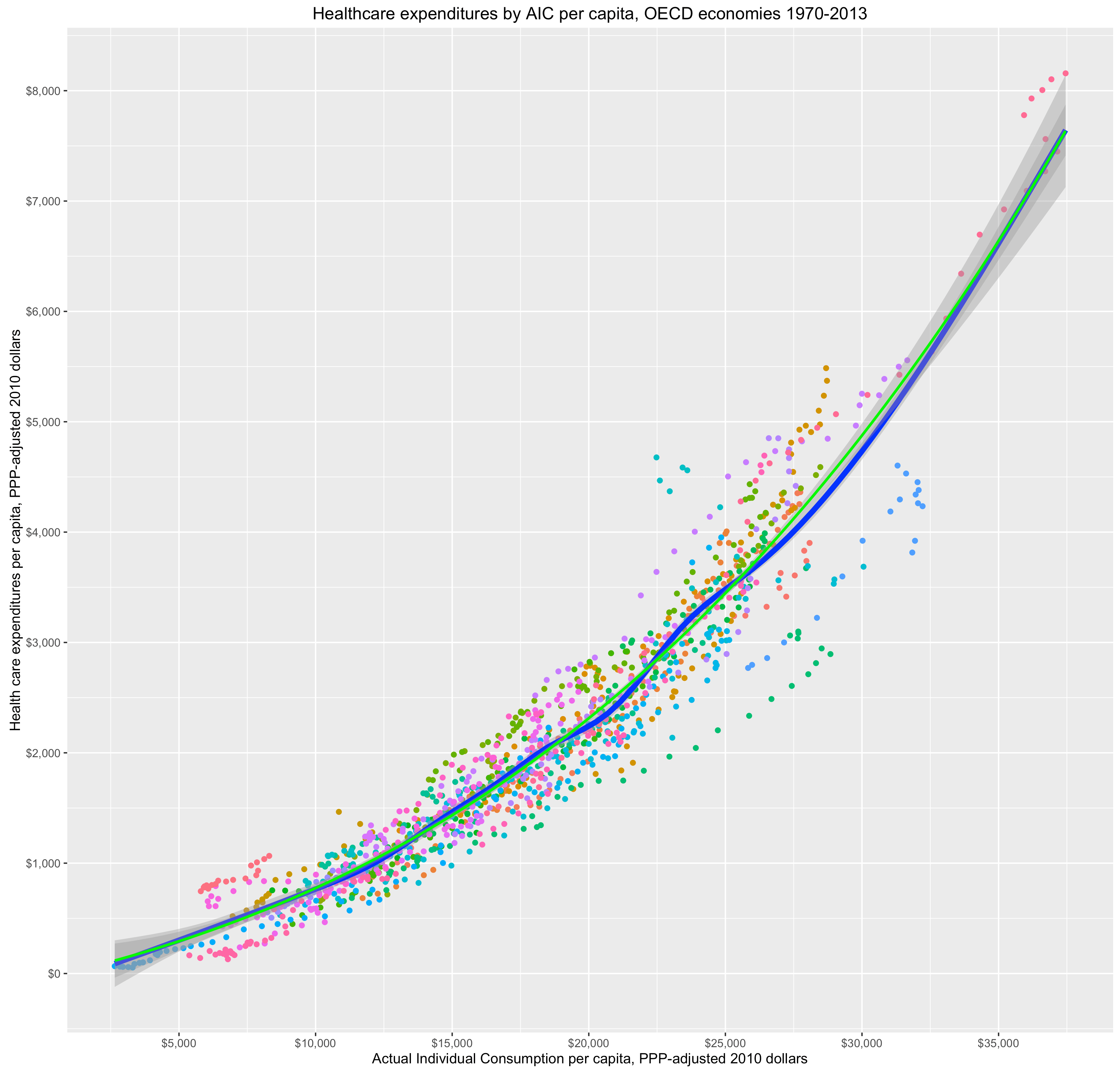
Note: the blue line is the loess smoother for the entire series whereas the green line is a 3rd degree polynomial, excluding US and Luxembourg from consideration, extended out across the entire plot (to include area covered by US etc). The lines look very similar and the US trend is quite close!
Alternatively, we can fit a 3rd degree polynomial across the entire series and view the progression by country.

The observed patterns by country are generally quite consistent with the polynomial trend, i.e., it does not look like this is purely an artifact of between country differences.
Or by year: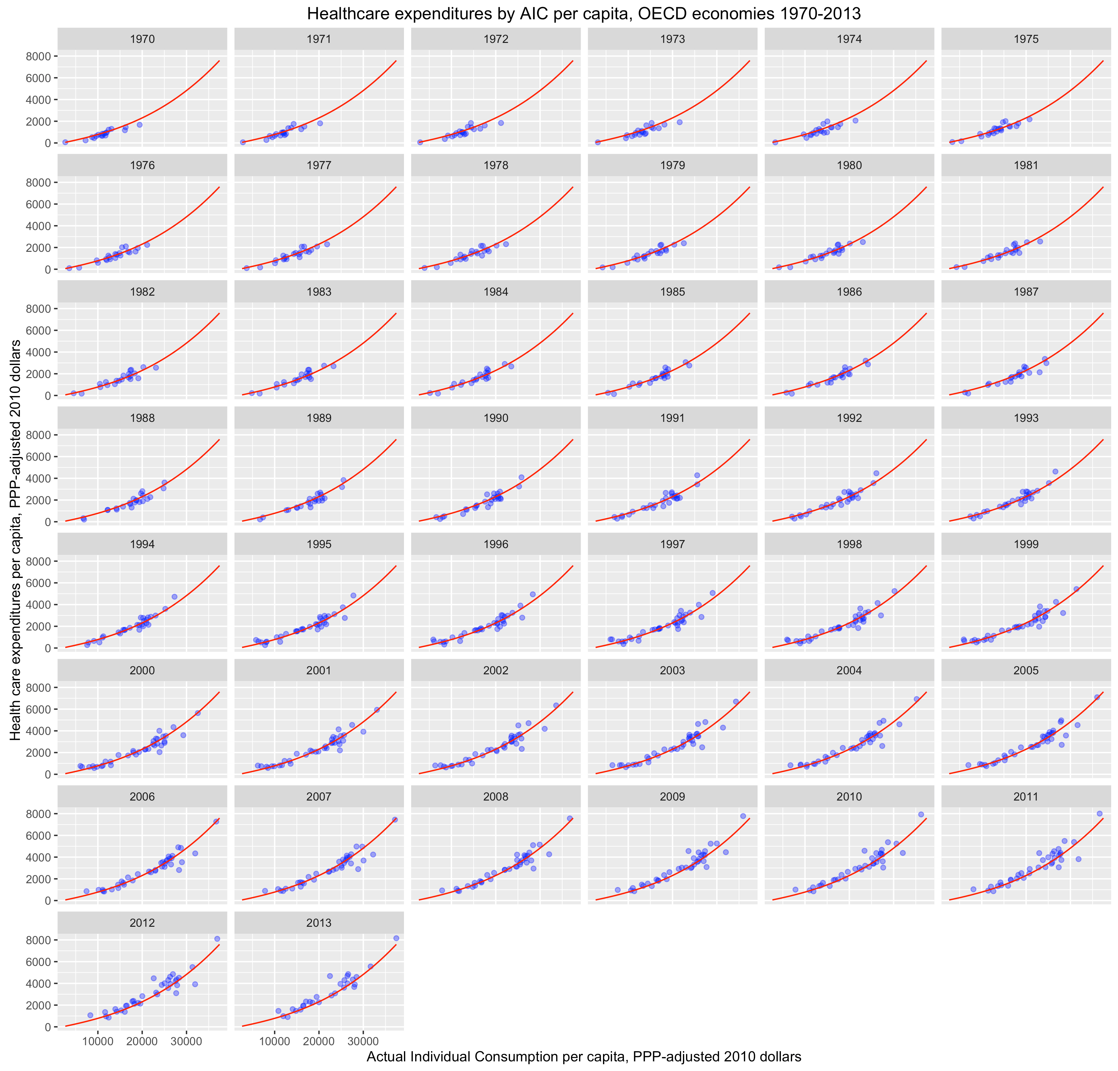
Now if I actually train these models on the reduced data set, i.e., excluding USA and LUX, you can observe that the polynomial models (2=2nd degree, 3=3rd degree) perform better than the linear specification (model 1). You can also see that the 2nd term in both polynomial specifications is quite clearly statistically significant too [all terms are highly significant with complete data set].

Even without year effects the polynomial models explains ~91% of the variation.
Now compare the model predictions on the full data set by year:

Note: The redline is the local trend within any given year whereas the black line corresponds to the actual-vs-predicted values (slope=1). You might note that, despite the fact I’m not correcting for year effects/time, the model generally holds up quite well, e.g., mostly falls very close to the overall expected slope across most years…..
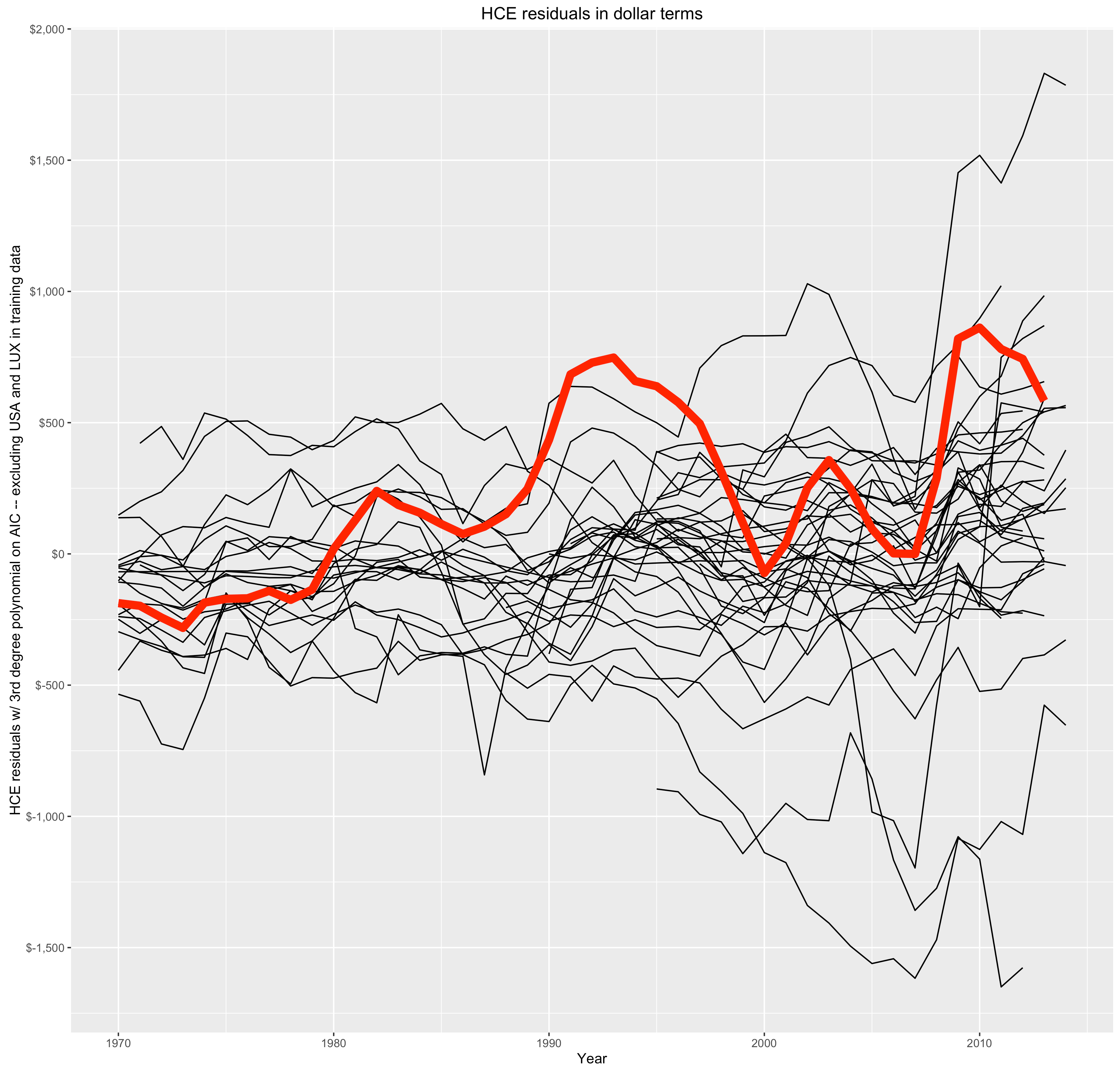

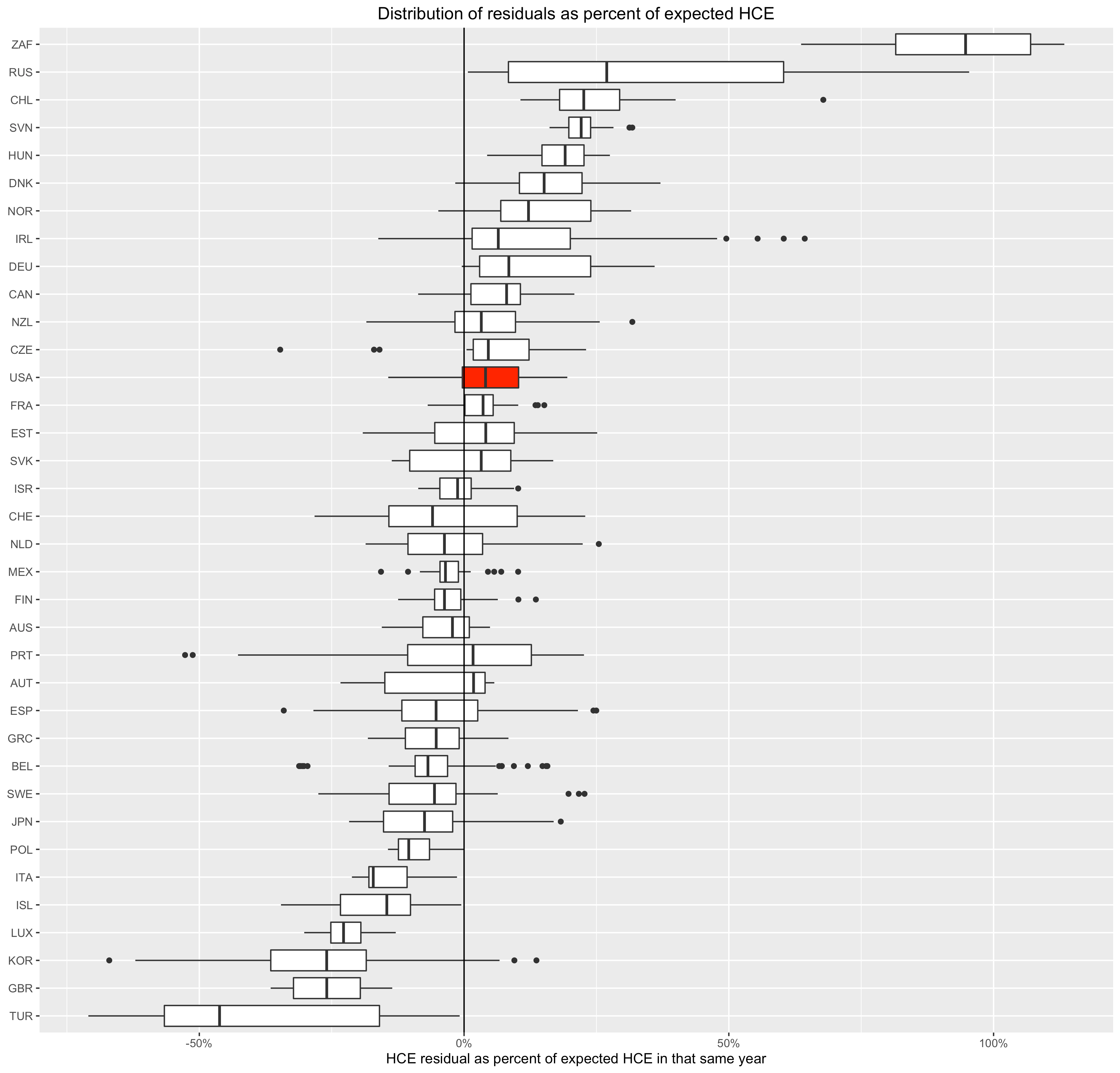
The US does not look like an outlier here.
The trend in annualized residuals appear to be modest, maybe 300 dollars over the course of 40+ years. This would tend to suggest that increasing material conditions can explain most of the observed increase in HCE amongst OECD countries over time.
I also found the polynomial model outperforms the linear model, both with and without year fixed effects (allowing the intercept for each year to vary independently), and that the 2nd polynomial term remains significant even with year FE.

Moreover, if I instead model the observation year as an integer, so that it behaves as a continuous variable, i.e., assuming an approximately continuous trend of increasing HCE across the board and thereby reducing the degrees of freedom significantly (relative to year FE), I get similar results, i.e., modest annual changes controlling for AIC and the polynomial model specification reduces the apparent effects of time (from, say, technological innovation) even more.

Along similar lines, if I explicitly include country fixed effects to crudely try to estimate the marginal influence of AIC within countries over time, I still find good evidence for non-linearity in the slope vis-a-vis AIC.

Alternatively, if I model HCE as a percentage of AIC including the USA and Luxembourg with country fixed effects:
Although this method has some issues (!!!), it still tends to suggest that there is a non-linear trend vis-a-vis AIC and HCE within countries even allowing for continuous growth in HCE over time. And if we actually peek at the country fixed effects in this model:
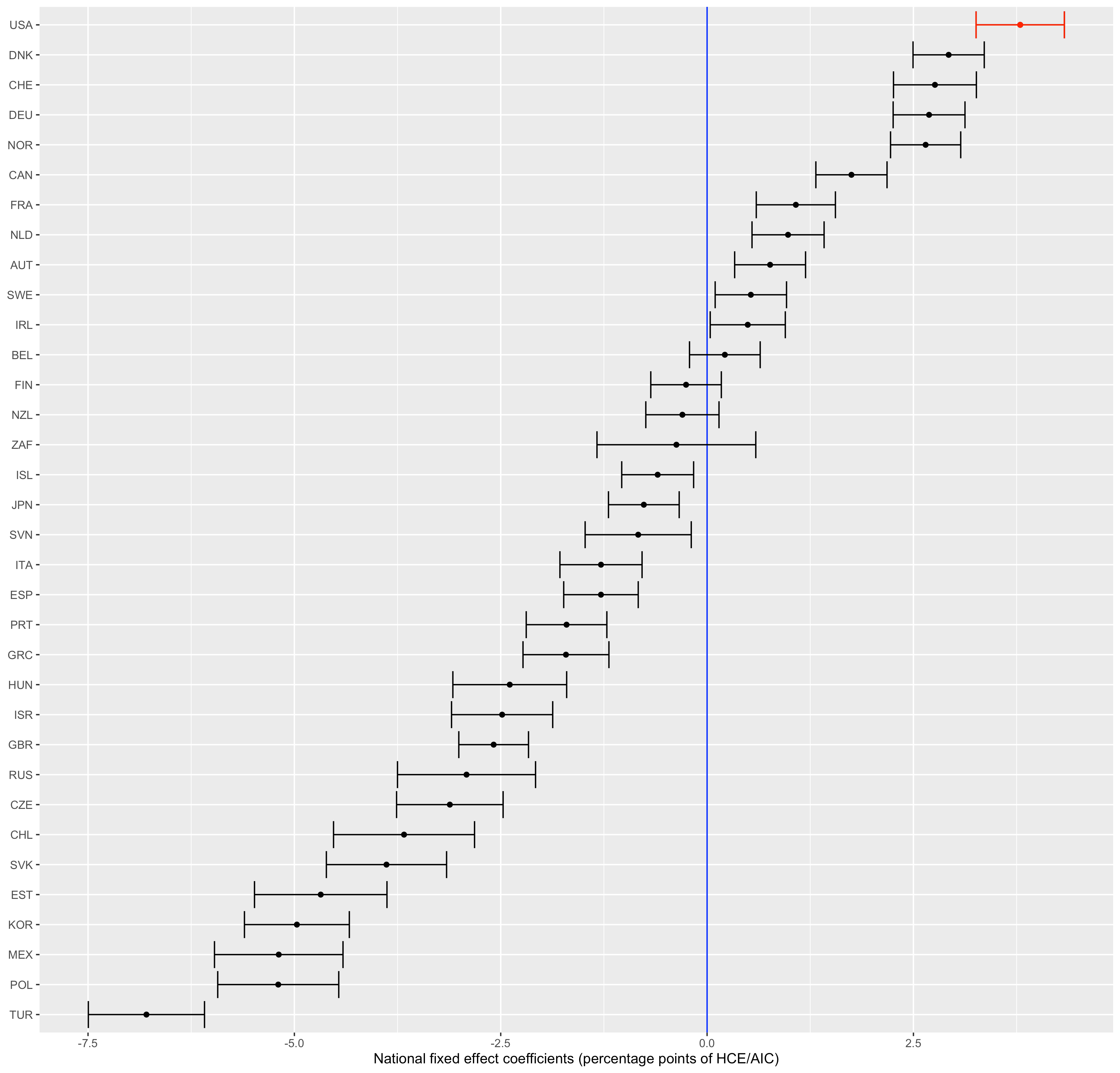
The US looks on a bit on the high side, BUT rich countries skew high systematically too!

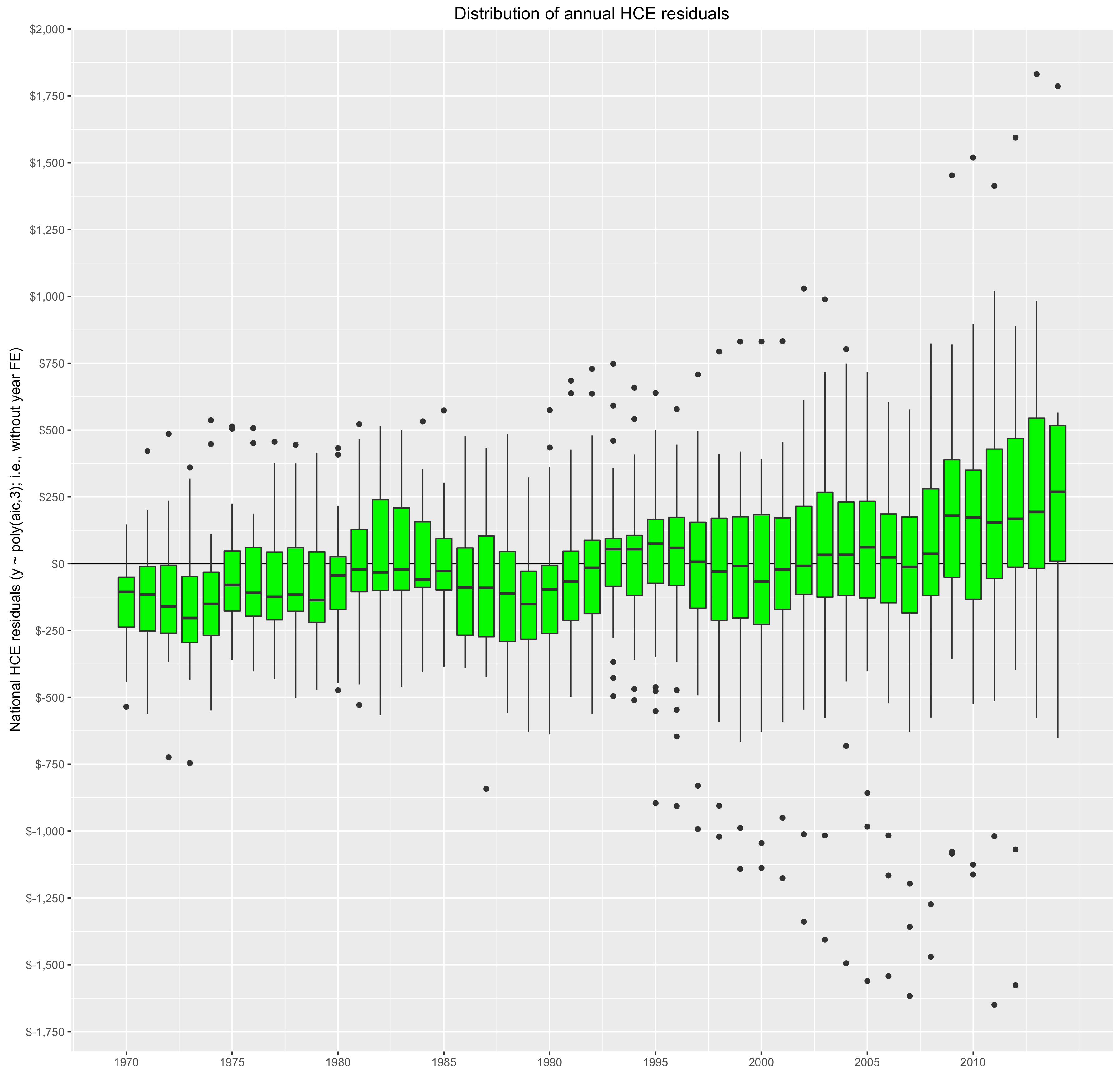
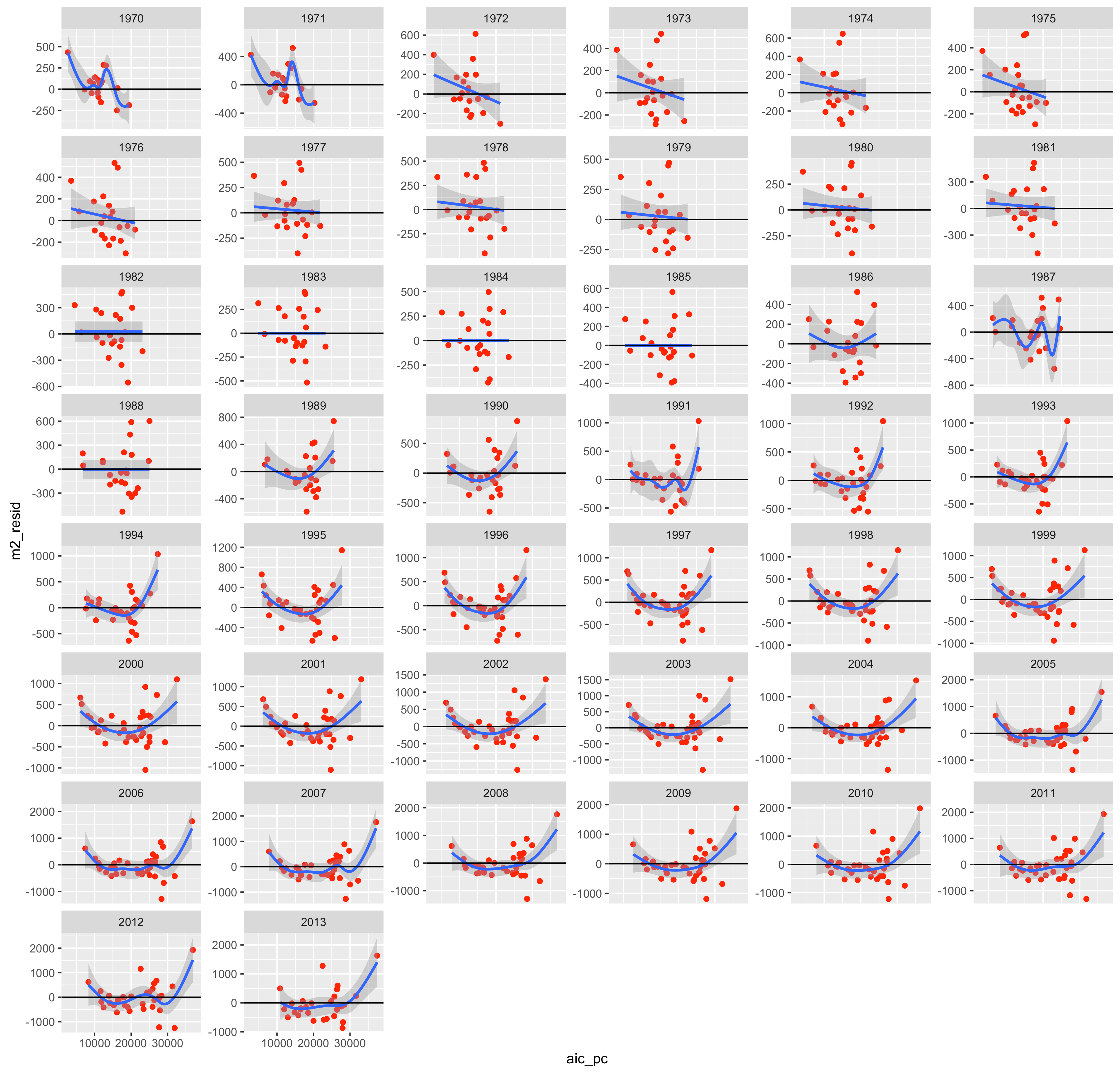
Another way to come at this issue is to look closely at the residuals in a linear model in several dimensions (e.g., across time, across differences in AIC, etc).
For instance, if I model this with year fixed effects and a constant slope for AIC:

With the year FE increasing somewhat:
This results in a strange looking U-shape:

Although that is about what I would expect given the apparent non-linear relationship with AIC and the particular distribution of AIC here.

Clearly this model has some significant systematic error if you look closely at it by AIC.
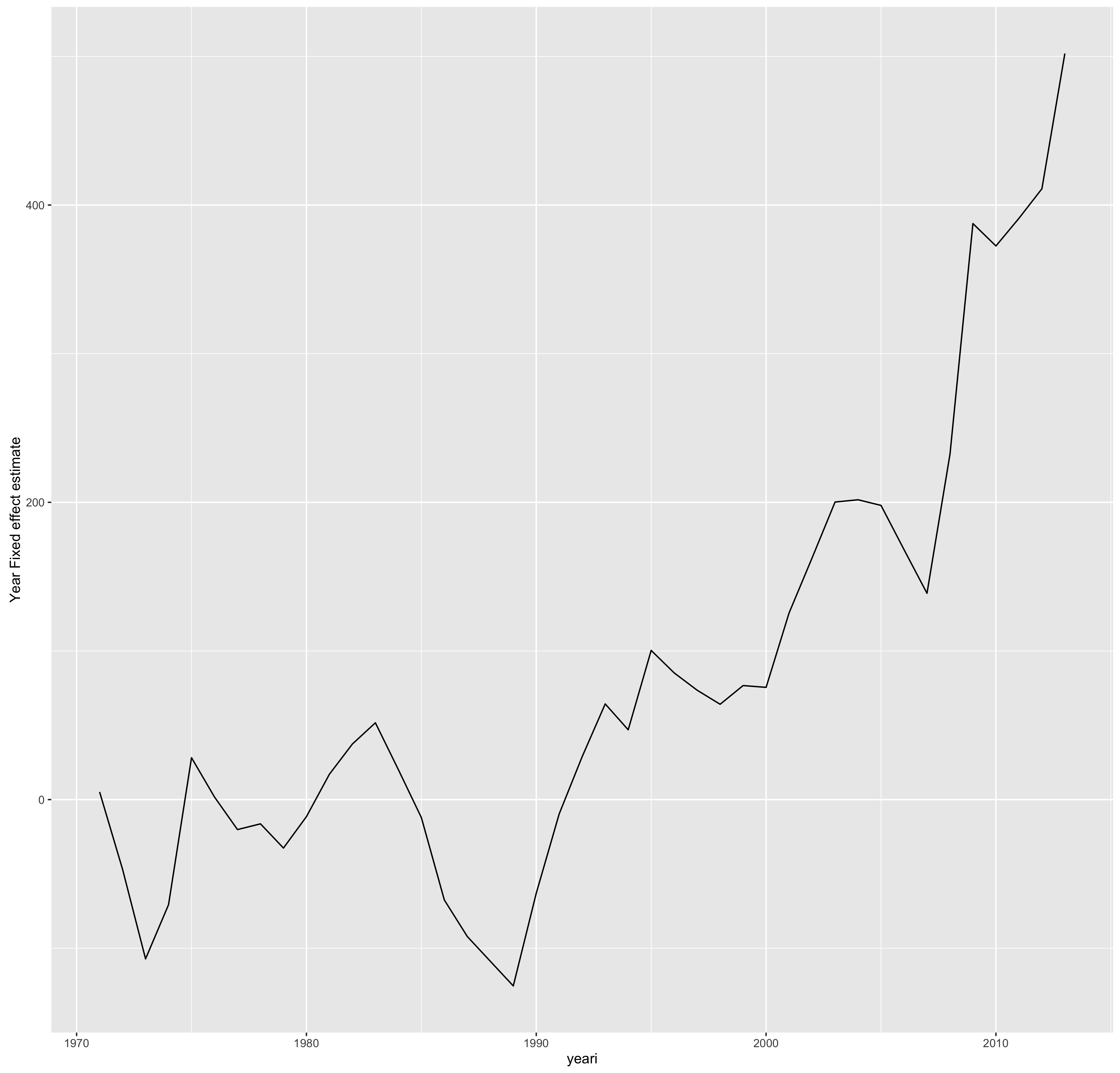
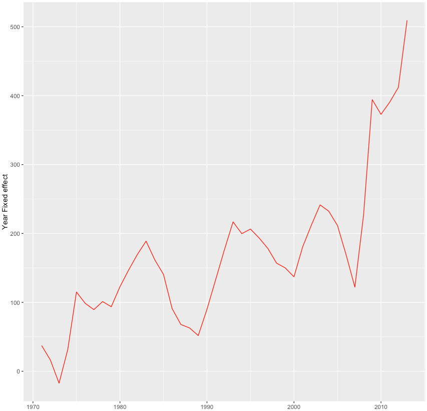
Alternatively, if I model this with a random effects model (lme4 package) wherein each year is allowed its own intercept and its own slope vis-a-vis AIC, I find the slope varies quite strongly with time.


In my opinion, this pattern needs to be explained by those that assert a strictly linear process. Why should the slope increase and the intercept decrease over time? (Has the return to expenditures vis-a-vis life expectancy, QALY, etc increased? I very much doubt it.)
This is entirely consistent with the polynomial model and a general trend of increasing AIC across most countries.
In any event, we can still pretty clearly see that these residuals are not distributed randomly vis-a-vis AIC.

Keep in mind that I don’t have these issues with the simplest polynomial model (excluding year effects)
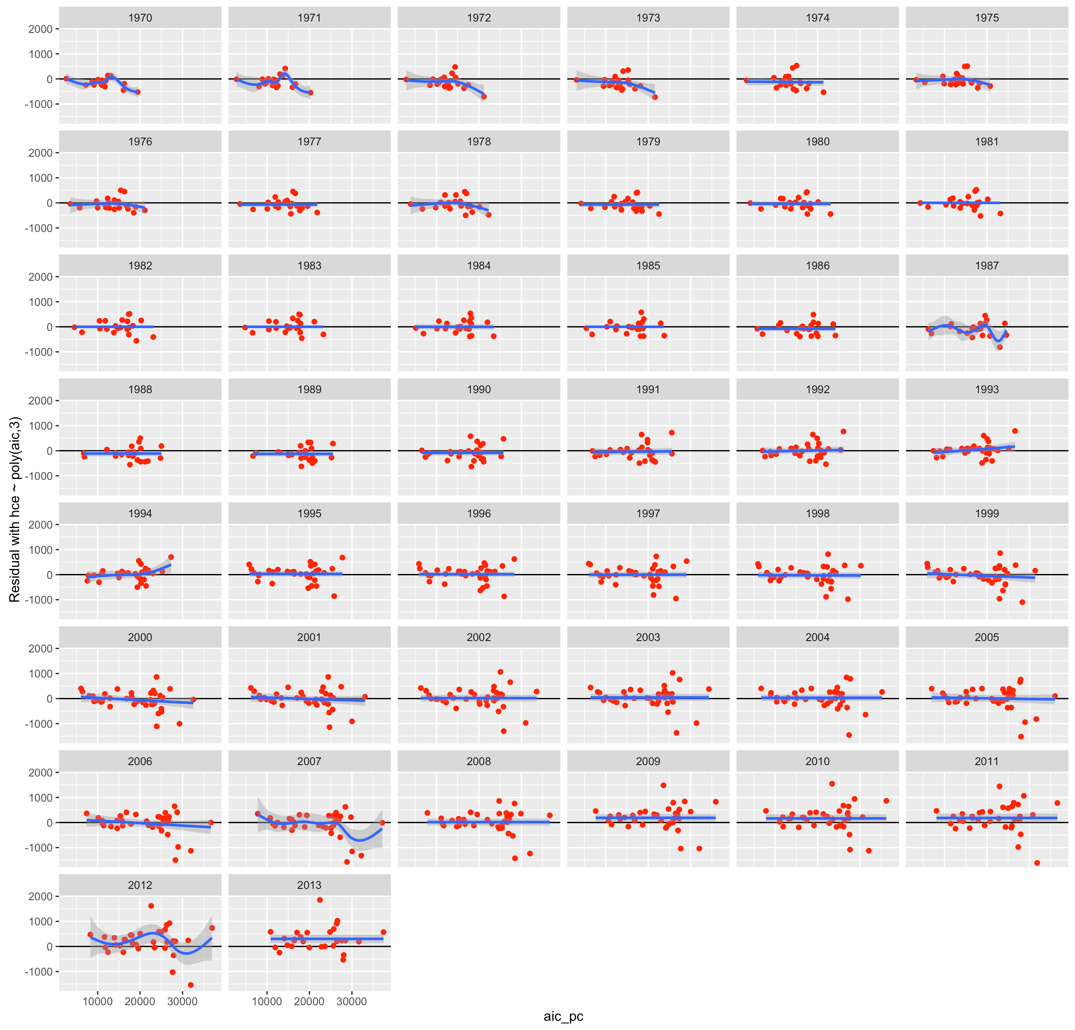
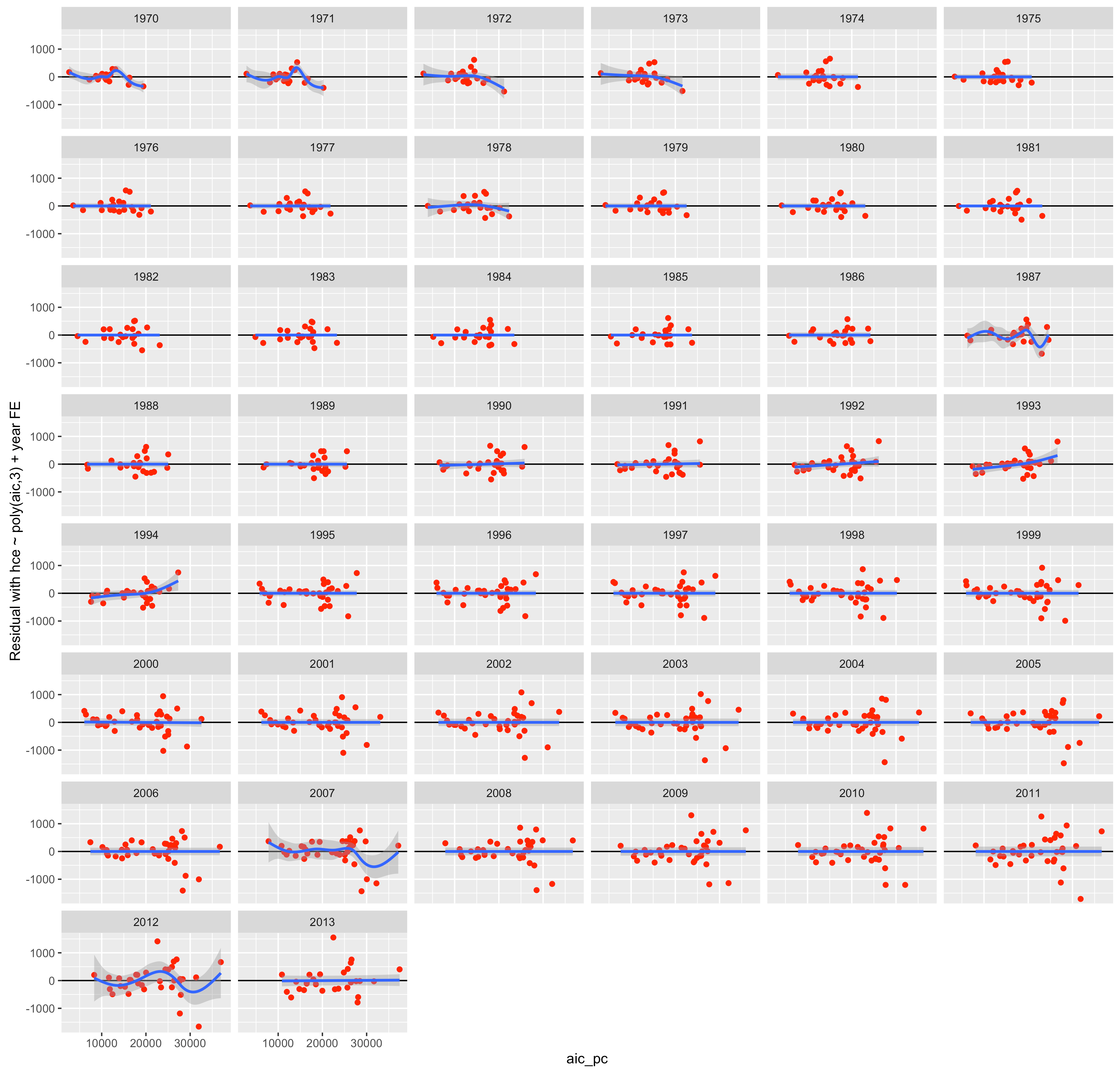
The actual intercept appears to shift slightly, but it’s not greatly skewed in any apparent systematic fashion. And if I include year FE in the model:
That’s about all I have for now.
In my view, this polynomial model is straight forward (few degrees of freedom), plausible, and most parsimoniously accommodates or otherwise “explains”:
- virtually all of the intra-temporal differences between countries
- large inter-temporal shifts in HCE amongst countries
- the broad global pattern of increasing health care expenditures
- fits rich AND poor countries in the same dataset quite well
If this HCE growth is primarily a consequence of inevitable pressure resulting from demand for technological improvements (medical devices, pharmaceuticals, surgical procedures, etc), why don’t we see proportionally similar increases amongst countries a decade or two behind us in economic development? If high US health expenditures are the product of lack of single-payer (limited market power etc etc), why did the US only really diverge relatively recently? (Did not similar differences in systems exist in the 70s or even early 80s?) If other developed countries have it figured out, why is their HCE increasing so rapidly and why is their trajectory so similar to ours vis-a-vis AIC per capita? If the relationship between HCE and AIC are truly linear in a given year, why should the overall slope change so much over time and why, even allowing for a substantial random slope, are these residuals non-linearly correlated with AIC (rich and poor countries skew high)? Why is the relationship in the much more economically diverse 2011 WHO/WorldBank data so clearly non-linear? (What explains this here, but not between OECD economies?)
In short: why is this not all much better explained as an overall non-linear relationship (as in the 3rd degree polynomial models above)?
Note: That is not to argue that technology had played no role here, I think it has, but it seems to be pretty modest as a root cause or independent predictor (as suggested by the annual coefficients ) as compared to the influence of increasing affluence in the US and abroad. Put differently, spending on new technology (or otherwise stimulated by it, e.g., diagnostics) may account for a significant fraction of the increase in spending in rich countries, but this doesn’t usually seem to happen all that significantly without a larger corresponding increase in broader consumption measures (i.e., even if you exclude HCE).
This is fascinating. A lot to think about and chew over. Thanks!🤔🙂