The Citizens for Tax Justice (CTJ) and Institute on Taxation and Economic Policy (ITEP), amongst other progressive organizations, have put forth the claim that our tax code is nearly flat on the basis that “regressive” consumption taxes in state/local tax codes offset federal and (to a lesser extent) state income tax progressivity.
The problem with almost all of these analysis is that they all invariably hinge on the fact that their reported ratios between consumption and income is greater than 1 at lower income levels. In other words, they are counting consumption taxes in the numerator that are not included in the income base (the denominator).
ITEP claims, in their description, that they’re correlating consumption patterns in the BLS’s Consumer Expenditure Survey to reported income. The problem with this approach is that the BLS CEX consistently indicates that the ratio between consumption to “income” exceeds 1 just shy of the 50th percentile on down (the bottom is >2x)
ITEP further papers over these flaws by effectively hiding non-linearity at negative numbers in their models (e.g., consumption 20x negative income).
Some money quotes on their model:
Our procedure for imputing consumption onto individual tax records can be thought of as involving two distinct steps: (i) econometrically estimating the necessary relationships for each of the desired consumption items from the Consumer Expenditure Survey (CES); and (ii) using the resulting regression coefficients to simulate consumption on the merged data file for non-dependents. Implicit in this approach is reliance on the strong separability of a utility function over different categories of consumption; i.e., we used a “utility tree” approach to estimate several systems of share equations.
…
Next, total non-durable consumption expenditures were imputed in a similar manner: separate ordinary least squares (OLS) regressions were estimated from the CES on both samples with a similar set of predictor variables. Coefficients from these equations were then used to impute mean (non-durable) consumption expenditures to each household and a normally distributed error term with a mean of zero and a standard deviation equal to the standard error of the regression was added to each imputed amount. Two sets of adjustments were then made to the imputed amounts.
First, the particular functional form used was unstable at very low levels of income resulting in extraordinary amounts of imputed consumption for several records. For nondurable consumption, our OLS specification included two terms, 1/Y and 1/Y2, where Y is total family income, that presented problems at both ends of the income distribution. For very low incomes, the nonlinearity introduced by 1/Y and 1/Y2 caused estimates of mean consumption to approach infinity. This was handled by constraining consumption for these records to be no more than 1.5 times income. This limit was based on analysis of the CES data independent of the imputation process.
Second, the tax return data that formed the basis of the income information for filers contained income amounts far outside the range observed on the CES and caused problems when our regression coefficients were used. Our approach was to assume that the estimated equation was valid for incomes within the range of the CES and to fit a spline function for the portion of income in excess of this amount for those households (about 2.5%) with reported incomes outside the range of that reported in the CES.
Without getting into the weeds with respect to how their model works (they don’t disclose nearly enough information or data to do this), I can reproduce their consumption tax numbers very closely by simply using the BLS CEX consumption to pre-tax income ratios and a flat consumption tax. In other words, you don’t need to assume that the poor are paying higher effective rates as a proportion of their consumption (e.g., on “sin” taxed goods) to get higher effective taxes as a percentage of this very limited definition of “income” on the poor. It’s quite clearly almost entirely a byproduct of methodological flaws that vastly overstate spending-to-income at low incomes and vastly understate spending-to-income at upper incomes.
You can reproduce my numbers using the BLS CEX tables [see incomes and higher incomes before taxes]
This one “fixes” the nonlinearity c-to-i ratio, like CTJ/ITEP do, for “very low” income at 1.5 (bottom two)

The “raw” data without the “fix” (albeit absolute value since average income is negative at the <5K/yr income range)
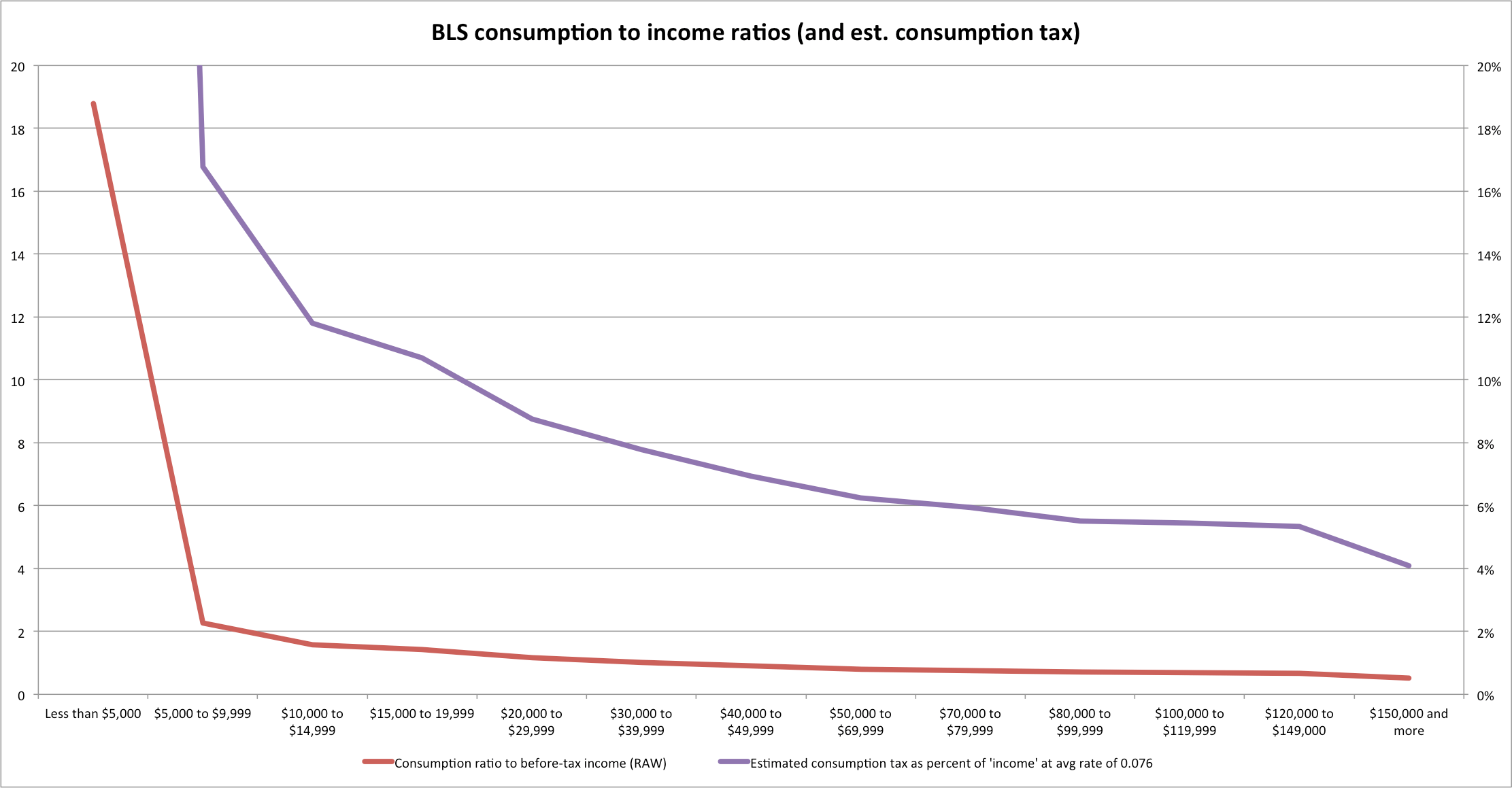
Long story short: consumption consistently not captured by “income” is driving almost all of these claims of large “regressivity” at the low-end (and probably significantly understanding consumption levels for middle to upper middle income people!)
Although there is certainly something to claims that excise and sin taxes hit the poor harder in proportional terms, these are a fairly small part of their comprehensive income and they’re probably offset by exclusions in many states for staples like groceries (which account for a larger part of low income households budgets). Net-net, the evidence I have seen leads me to believe that the fall-off in consumption taxes on upper income households is not nearly as large as it’s believed to be and it’s largely offset by state/local taxes on income….rendering a fairly flat “average” state/local tax burden and a (still) quite progressive tax code with federal taxes factored in.
Notes
Fed Paper: Is the Consumer Expenditure Survey Representative by Income?
The ratios of total expenditure to after-tax incomes by income shown in Figure 4 exhibit a dramatic pattern, and although there are some conceptual issues and systematic reporting errors with income taxes in the BLS tabulations, those sorts of corrections do not fundamentally change that pattern. The ratio of spending to income at low income levels seems implausibly high, and the ratio of spending to income at the top seems implausibly low. There are most likely problems with both income and expenditure reporting, and sorting households by income simply highlights those errors.
The bottom of the income distribution includes many households who under-report income (e.g., the self-employed), and hence, the high ratios of expenditure to income at low incomes can be partially explained by the presence of these households. The argument that income is missing at the bottom is reinforced by a pragmatic view of lower income households. It is impossible to spend twice your income (Figure 4) if you have no assets to draw down and no access to credit, which is the basic conclusion one takes away from wealth surveys like the SCF or Panel Survey of Income Dynamics (PSID).Thus, except for students, households with temporary business losses, and retirees drawing down assets, the high rates of implied dissaving by lower income households in the CE are already implausible, and proportional scaling up of spending would only increase these, already implausibly high, spending-to-income ratios.
It is also unrealistic to think that families above $100,000, on average, save the fraction of their disposable income implied by Figure 4, using it for purchasing stocks, bonds, and other investments that are not captured by the CE. Such behavior would yield average wealth to income ratios for higher income households that are much different than what we observe in wealth surveys (e.g., PSID and SCF).

P.S., To be perfectly clear: while it’s true that individual households or families can spend more than their income in any given year (e.g., by drawing down savings, borrowing, etc) and that same particular groups might save a large fraction of their income in any particular year, the size and historical durability of this phenemenon clearly indicates that the relationship between BLS reported “consumption” and reported “income” is substantially off for both high and low income households. It’s therefore silly to attempt to impute consumption taxes to households with these same obviously flawed ratios.
Update: another example of this ratio absurdity
Below is a chart showing average per person consumption and income (both pre- and post tax) as according to these very same BLS statistics [hint: richer consumer units are larger than small ones according to their data].
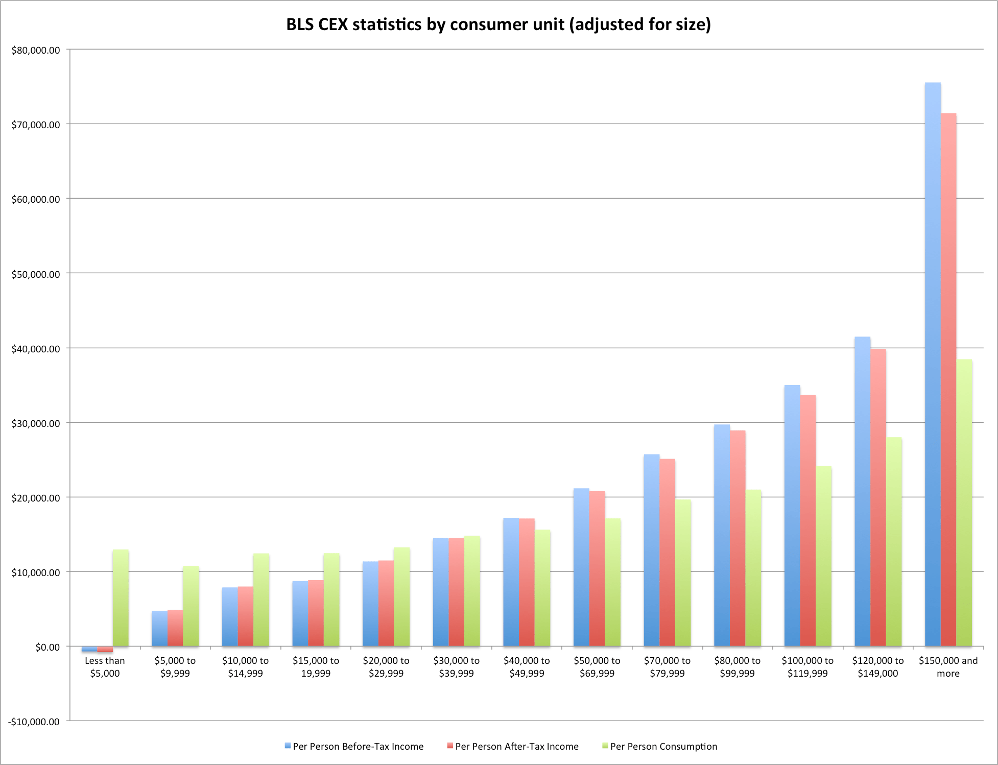
Compare, for instance, the 10-15K unit to the 50-70K consumer units. Can anyone really believe that despite an average per person “income” ~160% higher that they only spend ~38% more per person? Or that the highest income groups only spend 2-3 times as much as the very lowest on a per person basis…? REALLY???