Previously I demonstrated that actual individual consumption (AIC) is a superior predictor of national health expenditures (NHE) and largely explains high health spending in the United States.  Towards this point it is instructive to show that not only are health expenditures generally coordinated with AIC, but that all other major categories of expenditure are too, i.e., at given level of real consumption per capita all countries will tend to allocate their consumption quite similarly.

In this post I make extensive use of Principal Components Analysis (PCA) and related dimension reduction techniques to better characterize consumption patterns across several major categories of consumption in both the spatial and temporal dimensions.  I find that there is a latent factor that explains the great majority of the variance in consumption, that it is exceptionally well correlated with AIC, and that GDP has essentially zero incremental validity once we have accounted for AIC for practical purposes.  I also show that this factor holds up well to price adjustment for each consumption category and correlates similarly with AIC within the OECD.

Although my interest here is (was) largely in verifying my prior analysis as it pertains to health expenditures, i.e., that AIC is real, meaningful, and the measure we probably ought to prefer when discussing the efficacy of cost containment regimes, my analysis has broader implications.  For instance, it provides evidence (albeit in a roundabout fashion) that argues rather strongly against Scott Alexander’s widely cited post on cost disease, i.e., if health, education, construction, and so were truly uniquely expensive in the United States, the United States ought to stick out like a sore thumb in PCA and the like.  Instead what we found is that the US consumption patterns track well with its high overall level of real consumption (AIC).  Moreover, anticipating the argument that perhaps cost disease is simply well correlated with AIC, when we adjust for category specific price levels (i.e., “volumes”) we find PPP-adjusted AIC holds up very well in explaining the variance in the actual volumes consumed overall and that the US is, again, well on trend (which suggests actual apples-to-apples differences in cost are not the problem and actual increase in the quantity and quality of goods & services consumed in these categories drive most of the variance).

---

Broad international data (WorldBank ICP)

Intro

The World Bank helpfully maps these categories in their latest (2011) ICP report.

The shaded categories in the list below above are “nonhierarchical”-that is, they combine items outside of the hierarchical ICP classification (e.g., “education” combines the household expenditures on education with those of nonprofit institutions serving households and of the government). Categories not shaded are hierarchical.

(emphasis mine)

Note that columns 3-15 sum to AIC (column 2) and 3-14 alone in will get you very close (save mostly for small countries with high % tourism etc).

---

Analysis of real per capita expenditures

I will begin with the full ICP data set.

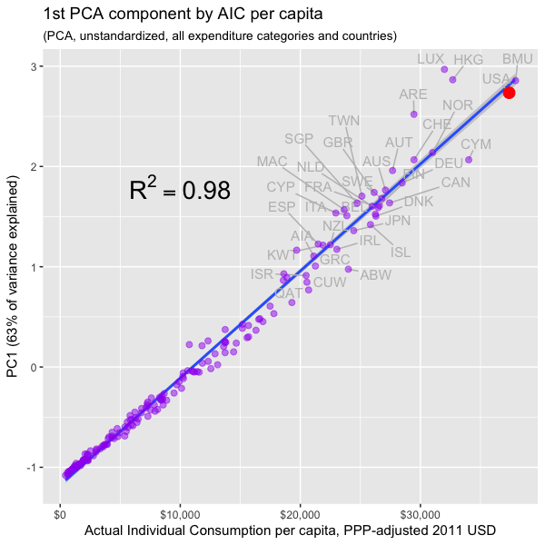
The factor scores generated by PCA for the first component are nearly perfectly correlated with AIC per capita.

Please note that all of these expenditures are computed on per capita PPP-adjusted figures that are standardized (think: z-scores) before being considered by the algorithm (it’s not as if this is simply sum of these expenditures).

This is telling us that:

1. there is an underlying structure in how countries allocate their consumption dollars between different categories of consumption that explains most of the variance
2. the primary component is exceptionally well correlated with AIC.
3. Different categories of consumption increase at markedly different rates as a function of AIC
4. US consumption patterns appear to be very consistent with its exceptionally high level of individual consumption (AIC)

PCA provides a useful backup to regressions on health expenditures here.  The algorithm is identifying the factors that best explain consumption across all of these different categories (not just health) and the first component it identifies, which explains the great majority of the variance, correlates nearly perfectly with comprehensive measures of individual consumption, not GDP.

If we plot factor scores for the first two components, some of these more unusual countries (e.g., Luxembourg and Bermuda) quite clearly pop out and the US still quite clearly clusters with more developed OECD countries (albeit further along the high consumption axis)

These scores are much less well correlated with GDP (especially for those countries where the disconnect between AIC and GDP is large– see Singapore, Qatar, etc)

Countries with high GDP and abnormally low consumption generally allocate their consumption in ways that are much more consistent with their overall level of consumption (i.e., much more like countries with much lower disposable incomes than their GDP might naively suggest).   This pattern isn’t only found with health care.

---

Expenditures as a share of consumption

Lest you think this is just a mechanical result of countries with high overall consumption spending more on nearly everything (despite prior conversion to z-scores etc), we also find these same patterns if we run PCA on these variables as a percentage of AIC and standardize them too (i.e., this is not weighted for the absolute proportion consumed)

The allocation of individual consumption expenditures generally correlates quite well with AIC and US is about where we would expect given the dispersion (note: some of these relationships are obviously non-linear and analyzing it in percentage terms tends to magnify the effects substantially — with non-linear dimension reduction methods this would likely tighten up considerably… a bit beyond the scope to include here).    The US also clusters with other developed countries in the 2nd component too.

GDP is comparatively poorly correlated with the 1st component.

Unsurprisingly, AIC fully mediates GDP’s association with these factor score in OLS.

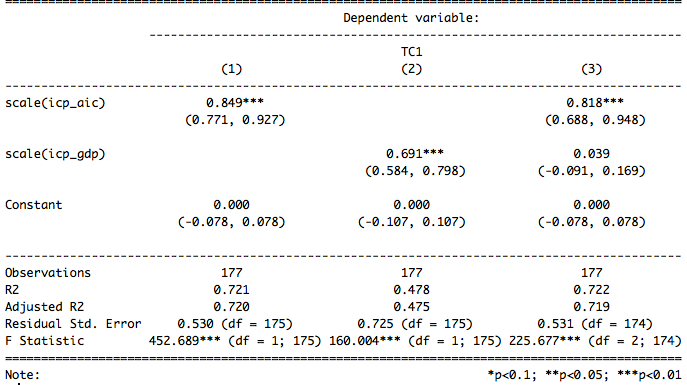
The allocation of comprehensive individual consumption expenditures (which includes health, education, social protection, etc) is much better predicted by AIC than GDP.

---

Consumption shares of subset

Likewise, even if we exclude health and education from consideration and look at the allocation across the remaining consumption areas in percentage terms, there is clearly a significant factor that correlates with AIC.  Simply knowing how countries allocate consumption across these categories we can predict AIC reasonably well.

Again, AIC fully mediates GDP.

---

More plots

Obviously we can also learn something about these patterns by simply plotting these expenditures out:

We can also crudely bin these categories together to make some of the underlying patterns a bit more self-evident:

Of course, large changes proportions does not imply an actual decrease in absolute terms.   Mostly the systematic change in proportional terms is a result of some categories increasing less rapidly than the overall real rate of increase in consumption.

---

Relatively highly-developed countries (OECD data)

Real per capita expenditures

The OECD supplies per capita volume estimates for each of these expenditure categories periodically, i.e., the nominal per capita expenditure is adjusted by the specific PPP for the expenditure category to produce a volume index (EU28 mean = 100).  Put differently, instead of merely adjusting for the average economy-wide PPP, which may over-state “real” consumption of (non-tradable) services in rich countries relative to (tradable) goods and is potentially (more) subject idiosyncratic price differences between countries, we can effectively remove these price differences and estimate the real quantities consumed per capita in each category (technically “volume” but it’s analogous to quantity, albeit there are varied items within each category).   If these patterns were merely produced by systematic price differences and these OECD PPP are competently estimated (I generally think they are), then doing PCA or factor analysis on these adjusted expenditure categories should produce much less impressive results.

This tends to suggest that the PPP-adjusted AIC per capita is a good representation of how much real (non-collective) consumption happens across the OECD at least, i.e., unusually high costs for health care, education, etc generally aren’t causing AIC to present a misleading impression of material living conditions.

Obviously, the association with GDP runs entirely through AIC (I won’t waste space here with OLS etc).

Even if I go so far as to entirely remove health, education, and transport from PCA consideration (presumably some areas that might skew US consumption in popular imagination), we get much the same results!

And in case it’s not sufficiently obvious, the association between GDP and these factor scores is entirely mediated by AIC.

Consumption patterns at multiple levels of analysis are best explained by AIC (and likely gross-adjusted household disposable income), not GDP.   This may seem obvious, nearly tautological, but given that AIC is the total comprehensive individual consumption by definition, consider that if it also fully mediates GDP with respect to the allocations between specific categories it makes little sense to prefer to reason about specific consumption allocations relative to GDP when we have much better measures available for these purposes (e.g., AIC, household disposable income, etc).

---

Analysis without standardizing (scaling) variables

Both PCA and factor analysis are sensitive to the scaling of the variables.  It is usually standard practice to standardize the variables to z-scores because the natural units of the predictors often are not comparable.  In this case, these variables generally are since they’re all measured in PPP-adjusted dollars (though the actual category specific price levels may vary somewhat between countries).  By running this on unstandardized variables we’re asking a slightly different question, i.e., what best explains the overall variance in dollar-weighted terms.  Both are useful in their own way.

Again we find the first component (72% of variance) is exceptionally well correlated with AIC and that the US is pretty close to trend.

We can also plot the first two components to see how different countries shake out

It is quite apparent here that some of these more abnormal economies with high tourism, large non-resident workforce, etc show skewed consumption patterns, i.e., a disproportionate share of their consumption is in housing, energy, non-resident consumption, etc.  See those countries in the bottom left quadrant or those generally away from the generally more developed cluster of countries.  US is pretty much where I would expect it to be, i.e., clustered with N/W Europe etc but even further out due to overall higher consumption and higher disposable incomes.

AIC appears to be roughly orthogonal to the 2nd component overall, but it seems pretty clear this is due to a few of the rich countries with abnormal consumption behaviors confusing the patterns.  Plotting more comparable countries, roughly the OECD, (the dotted line) we can see this a bit more clearly.

PC2 is largely a corrective to these expenditures as they relate to AIC.  If we were to delete these abnormal countries and re-run PCA on the resulting data PC1 would correlate even better with AIC and would surely load even more on health, misc. goods & services, recreation and culture, etc.

Across both components these US is further out in a way that is very much consistent with its high material standard of living.  If health expenditures were actually consuming an abnormal share of consumption (and thus other components also lower) I would expect the US to be well off trend across at least one of these axes as some of these other countries with obvious unique aspects to their economy are.

---

This also works as a time series (OECD)

Using household and government final expenditures from the OECD I can closely approximate the individual consumption by category as above as a time series (lumping some small amount of collective consumption contained within government accounts for health, education, and recreation and culture into their respective totals since not enough countries break this out in detailed format to do it in a way that is 100% compliant with AIC tabulation requirements)

Note: Classifications of household and government expenditure are described here if you are curious about what each category entails.  Also the breakdown of “individual” vs “collective” consumption by government is described on page 191 of SNA 2008 manual.

Though there may idiosyncratic differences between countries in specific categories, there tends to be much similarity at similar AIC and in the long run there is significant convergence across countries.  This even seems to hold across time, as in, AIC of 20,000/person in PPP-adjusted dollars in 1980 is very similar to the same PPP-adjusted amount in 2010 in terms of the allocation across different expenditure categories.  Some categories seem to have moved modestly in ways that are not explained by AIC (e.g., communications with the growth in technology), but mostly these patterns are well explained in both the spatial and temporal dimensions by AIC.

I get much the same result with unstandardized PCA, i.e., the first component is nearly perfectly correlated with AIC.

The 2nd component is mostly orthogonal to both AIC and health.  It seems to pertain to the balance of tourism and overseas buying, which re-allocates consumption across several categories here (whereas AIC takes the net effect of these into reasonable account so overall there’s not much effect), and the US is fairly neutral here.

Amongst those categories that are well associated with material affluence the United States is well represented and about where we’d would expect based on AIC (usually at or amongst the highest).

---

AIC also correlates better with each consumption category

AIC correlates better with each consumption category individually regardless of method, transformation, etc (with few exceptions).

Note: Spearman with log transforms are perfectly identical to linear (no effect on rank ordering), so I excluded them to save space.

Reminder: The SNA health category does not match the WHO health estimates (WHO NHE estimates tend to be more comprehensive (larger) and be more consistent with high elasticities with respect to income, consumption, etc).

---

AIC mediates GDP (especially the non-AIC parts of GDP)

AIC tends to mediate GDP in OLS for each expenditure category (especially those that reflect actual resident consumption instead of “consumption” expenditures on behalf of tourists, non-resident workforce, etc).

Likewise, if we subtract AIC from GDP, so as to get a cleaner estimate of the actual effect of things like net exports, gross fixed capital formation, collective consumption, etc, we find that they predict little.

And similar results from an ordinal regression model (better handling of non-linearity and more resistant to outliers)

---

Conclusion

It may seem obvious to many people that once we have accounted for comprehensive measures of household consumption like AIC that other components of GDP (e.g., net exports, gross fixed capital formation, collective consumption, etc) have virtually zero marginal informational content vis-a-vis the absolute quantities or the allocation of expenditures across consumption categories (especially that of residents vs tourists, non-resident workers, etc), but this is not just about consumption per se.

AIC is also very well correlated with comprehensive measures of household disposable income and yields very similar answers as it pertains to national health expenditures and similar questions.   Gross adjusted household disposable income is little more than AIC plus household savings:

source

There is a fairly predictable long run relationship between household consumption and disposable income when aggregated at this level of analysis (long run in the sense that households may smooth consumption in the short run out of savings or by incurring debt).   AIC happens to be more readily available in more places than similarly comprehensive measures of household disposable income and is a less volatile indicator due to consumption smoothing behaviors, but I would fully expect this factor of consumption to correlate quite similarly with disposable income as it does with AIC even though there may be some modest differences in marginal propensity to consume between countries in these terms given endogenous differences, access to credit, etc.

Put differently, AIC is both a very powerful indicator in its own right (i.e., willingness and ability to consume on the margins where it may differ from disposable income) and it’s also an much better proxy for the economic situation of the actual household sector (e.g., household disposable income) than GDP as GDP can and does diverge quite substantially for multiple reasons.  I am going to liberally quote from a report on economic measurement issues authored by Joseph Stiglitz, Amartya Sen, and others since it speaks the limitations of GDP and some of my preferred measures (AIC and HH disposable income):

Gross domestic product (GDP) is the most widely used measure of economic activity. There are international standards for its calculation and much thought has gone into its statistical and conceptual bases. But GDP is a measure of mainly market production (products that are either exchanged through market transactions or produced with inputs purchased on the market), and thus more geared to measure the aggregate supply side of economies than the living standards of its citizens. Although GDP levels are correlated with many indicators of living standards, the correlation is not universal and tends to become weaker when particular sectors of the economy are concerned. For example, real household income – an income measure which is more closely related to living standards – has evolved quite differently from GDP growth in a number of OECD countries. Too much emphasis on GDP as the unique benchmark can lead to misleading indications about how well-off people are and run the risk of leading to the wrong policy decisions. The purpose of this chapter is to go beyond GDP in our quest for better economic measures of living standards. At the same time we shall be looking for indicators that remain within the broad boundaries of a national accounting framework.

[snip]

3 – A first step: emphasizing national accounts aggregates other than GDP

3.1. Taking account of depreciation and depletion

24. GDP is a measure of the amount of final goods and services produced within a country in a year (or a quarter). Gross output measures take no account of depreciation of capital goods. But if a large amount of output produced has to be set aside to renew machines and other capital goods, society’s ability to consume is less than it would have been if only a small amount of set-aside were needed. Thus, an immediate adjustment to GDP is to account for depreciation; doing so, leads to a measure of net domestic product (NDP). Thus, net measures should be emphasized over gross measures of economic activity when the objective is to track standards of living.

[snip]

3.2. Domestic and national income

31. Although we have been referring to net product, it is more relevant (from a perspective of economic well-being) to refer to net income. ‘Product’ relates to the supply side of the economy whereas ‘income’ refers to the ultimate purpose of production, namely use for consumption and higher standards of living. In what follows, we shall therefore reason in terms of ‘income’ rather than ‘product’. When turning to real income as opposed to its money value, a question arises on how to deflate nominal values. Whereas ‘product’ is typically expressed as the quantity or volume of goods and services produced, real income expresses the quantity of products that can be purchased with a given sum of money income. Before turning to the measurement of real income, additional adjustments will be discussed that can be brought to the measure of net (nominal or monetary) income.

32. Globalization may lead to large differences between measures of the income of a country and measures of its production. The former is more relevant to peoples’ living standards because some of the income generated in production by residents is sent abroad, and some residents receive income from abroad. Consequently, a more relevant measure than GDP and NDP, in our search for a measure of living standards, is net national disposable income (NNDI, see Box 1). This measure accounts for payments and receipts of income to and from abroad. This too is a standard variable in countries’ national accounts.

33. As production shifts from manufacturing to services, the differences between GDP and NNDI has increased in some countries. This affects the judgments of how well off people are. Assume, for instance, that more and more production occurs inside a country by firms owned abroad.  While the profits generated by these firms are included in GDP, they do not enhance the spending power of the citizens of the country. For citizens of a poor developing country, to be told that GDP has gone up may be of little relevance; they want to know about their own living standards. This is especially the case in those countries relying heavily on mining or oil, which may receive a small royalty but where most of the returns accrue to the headquarters of a multinational company.  Even among relatively wealthy OECD countries, the gap between NNDI and GDP can be of importance, as Figure 2: Net national disposable income as percentage of gross domestic product shows in the case of Ireland. There, the declining share of NNDI in GDP reflects the large foreign direct investments in the economy and the large profits that are transferred outside of Ireland. By this measure, Irish income has increased by less than GDP growth would have suggested.

[snip]

35. Taking these changes in relative prices into account, along with real international transfers and real depreciation, yields a measure of real net national income for the entire economy. The figures below show that there is little to report home about the difference between constant price GDP and real net disposable income for some countries – the United States and France being cases in point. However, the example from Norway suggests that international price changes can drive a significant wedge between volume GDP and real income.  Norway’s economy and real income benefited enormously from rising oil prices until 2008, allowing Norwegians to buy more imports for the same amount of oil exported. This is reflected in the more rapid rise of real net disposable income compared to that of GDP at constant prices. The measurement effect comes through because real NNDI is obtained by applying a price index for final domestic demand (final consumption and investment), part of which is imported. Note, however, that the ‘net’ calculation that underlies the Norwegian income measure does not reflect the depletion of Norwegian subsoil resources.

3.4. Defensive expenditures

48. Expenditures required to maintain consumption levels or the functioning of society could be viewed as intermediate inputs – i.e. these expenditures confer no direct benefit. Many such ‘defensive expenditures’ are incurred by government, others are incurred by the private sector. For example, expenditure on prisons could be considered a government incurred defensive expenditure, and expenditures on commuting to work are an example of privately-incurred defensive expenditures. Several authors suggested treating these expenditures as intermediate rather than final products, hence excluding them from GDP.

49. At the same time, difficulties abound when it comes to identifying which expenditures are ‘defensive’, which are not and how to treat them in national accounts. What are possible ways forward? Options include:

First, focus on household consumption rather than total consumption. For many purposes, this can be a meaningful variable. All of government consumption expenditures (such as prisons, military expenditures or the clean-up of oil spills) are excluded from households’ final consumption. If one wants to capture ‘individual consumption’ provided by government, the SNA measure of actual final household consumption is appropriate because it captures these services provided by government (government ‘collective consumption’ is never imputed to households). This distinction between individual and collective consumption follows directly from the second criteria proposed by Kuznets (see Box) to distinguish between final and intermediate consumption of government services.

[snip]

50. One consideration may help to decide whether collective non-market services provided by general government should be considered as intermediate consumption or as investment. By definition, intermediate consumption is an input into production that is used up within the accounting period. Collective services like national defence or security are conditions of economic activity but, clearly, they are not “used up” during the accounting period. Moreover, as non-rival and non-exclusive public goods, they can benefit many processes of production at one time. To this extent, collective services better fit the definition of an (intangible) fixed asset. In order to make clear that this type of assets can be used simultaneously by all agents in the economy, a notion of collective investment, indicating the propriety of society as a whole on these assets, could be introduced.

4 – Second step: the household perspective

64. Much of the public discussion about living standards focuses on indicators for the entire economy, and more often than not GDP.  But, in the end, it is individuals whose economic situation should be assessed when talking about the standard of living. A glance at the evolution of the real income of households and the volume change in GDP (Figure 7: Real household disposable income and GDP Percentage growth at annual rate, 1996-2006) confirms that in general, one is not a good substitute for the other. Although in some countries real disposable income by households closely tracks volume GDP growth, there are many examples where this is not the case – Italy, Japan, Korea, Poland, Slovakia, Germany – to name a few.

[snip]

66. Measures of real household income appear to be suitable for this purpose. Earlier on, we discussed some of the income concepts for entire economies (national income, disposable income etc.). These income categories can also be computed for private households. In so doing, the re-distribution of income flows between economic sectors need to be taken into account. For example, some of the income of citizens is taken away in the form of taxes: this is money that is not at their disposal. Conversely, households receive payments from government and this must be added to their income. Households also receive and pay property income, for instance dividends paid out by corporations and mortgage interest paid to banks. When all these monetary flows are taken into account, one ends up with a measure of household disposable income.
67. In a world of perfect, symmetric information and efficient markets, it could be argued that households see through the ‘sectoral veil’ and account, for instance, for the fact that eventually corporations are owned by households and that government expenditure now may lead to future taxes. But perfect information is an unrealistic assumption and more often than not, households will simply look at their income and wealth in judging their economic situation and their consumption possibilities.

68. While disposable income is a useful statistic, it suffers from an important asymmetry. Some of the money that government collects from citizens via taxes is used to provide public goods and services, and to invest in infrastructure. While disposable income measures add and subtract transfer payments between sectors, no adjustment is made for the value of the goods and services provided by government to households in return for the taxes they paid. When an adjustment is made for the value of goods and services received, one obtains a measure of adjusted disposable income. Similar to the adjustment of disposable income, an adjustment for government-provided services can be made to household consumption. This leads to a measure that has been labeled actual final consumption by households [NOTE: This is identical to AIC]

4.1. Adjusting income and consumption measures for government services provided in kind

69. The invariance principle mentioned earlier implies that a movement of an activity from the public to the private sector, or vice versa, should not change our measure of economic performance, unless the switch between public and private provision affects quality of the service or access to it. This is where a purely market-based measure of income meets its limits, and where a measure that corrects for differences in institutional set-up may be warranted for comparisons over time or across countries. Adjusted household disposable income and actual final consumption are measures that go some way towards accommodating the invariance principle, at least where ‘social transfers in kind’ by government are concerned. These measures are computed by adding to household income and to household consumption expenditure the equivalent of the goods and services provided in kind by the government (Box 6).

70. The meaning of adjusted disposable income is best explained by way of an example Table 2….  [cut for brevity]

Both AIC (also known as “actual final consumption”) and adjusted household disposable income are invariant to public vs private sector arrangements and they are closely related (AIC + HH Savings = adjusted HH disposable income).  By preferentially using these measures we sidestep most/all of the aforementioned issues with GDP to arrive at a purer reflection of average material wellbeing that is not likely to be substantially biased by differences in how different sorts of countries provision services like health, education, etc.  [On a related note there is also a variety of literature showing that consumption in and of itself is a stronger predictor of well being than “income” (both micro and macro) and tends to be better correlated with life expectancy, SDI, etc than GDP at least]

My analysis with PCA and related methods earlier in this post suggests that PPP-adjusted AIC successfully captures something quite fundamental about the material living conditions of countries (or at least to a much greater degree than does GDP) and that there is tremendous consistency in how countries of similar AIC choose to allocate their consumption expenditures (especially without the presence of large “external” distortions in the form of tourism, non-resident workforce, etc that skew the allocation across expenditure categories even while leaving AIC itself relatively unaffected).  This also seems to work quite well in the temporal dimension.

In short:

1. the patterns I identified with health expenditures and AIC (relative to GDP) are found with essentially all major consumption categories.
2. there are good theoretical reasons to expect these consumption expenditures to interrelate to each other in the manner that they do
3. the first component, the latent variable, that best describes the variance in multiple PCA analyses is exceptionally strongly correlated with AIC and it explains most of the variance.
4. all of the dimension reductions I ran on expenditures suggest US patterns are very much consistent with what we would expect from a country of its AIC [certainly not wildly different as we should surely expect if “cost disease” were some uniquely American phenomenon with far reaching consequences]
5. similar patterns almost certainly exist with respect to adjusted household disposable income too

Given all of this, when US AIC pulled further away from the OECD starting around mid-80s it likely reflected a very real and meaningful change in material living conditions relative to the most of the OECD.  I would very much expect health and other areas of consumption to reflect this fact.  Likewise, I would expect those countries experiencing AIC that the US experienced decades earlier to allocate quite similarly, as in, AIC of ~31K in the US in ~1995 is going to look quite a bit like AIC of ~31K in Norway ~15 years later in terms of the proportions and actual expenditures on major expenditure categories like health, recreation and culture, miscellaneous goods and services, and so on (and even more so in larger countries where spending abroad is less viable and less attractive).

Incidentally, RE: “cost disease” themes, although the correlation between AIC and per capita education expenditures is fairly modest (or at least it is as tabulated at the level of national accounts), this is likely due in large part to different age structure (which does not have much effect on NHE) and, to lesser extent, different participation rates.  Amongst OECD countries there is a pretty significant correlation for per pupil/student expenditures and AIC per capita:

source

[and I suspect this this would tighten up further with a better accounting of benefits etc]